Premium
 Download
Edit
Download
Edit
Download the Informal Comparative Inference Facts & Worksheets
Click the button below to get instant access to these worksheets for use in the classroom or at a home.
Download This Worksheet
This download is exclusively for KidsKonnect Premium members!
To download this worksheet, click the button below to signup (it only takes a minute) and you'll be brought right back to this page to start the download!
Sign Me Up
Edit This Worksheet
Editing resources is available exclusively for KidsKonnect Premium members.
To edit this worksheet, click the button below to signup (it only takes a minute) and you'll be brought right back to this page to start editing!
Sign Up
Not ready to purchase a subscription? Click to download the free sample version Download sample
Download This Sample
This sample is exclusively for KidsKonnect members!
To download this worksheet, click the button below to signup for free (it only takes a minute) and you'll be brought right back to this page to start the download!
Sign Me Up
Table of Contents
In this lesson, students will be able to draw informal comparative inferences about two populations. They will informally assess the degree of visual overlap of two numerical data distributions with similar variabilities, measuring the difference between the centers by expressing it as a multiple of a measure of variability. Moreover, they will expand their knowledge on the use of measures of center and measures of variability for numerical data.
See the fact file below for more information on the informal comparative inferences or alternatively, you can download our 33-page Informal Comparative Inference worksheet pack to utilise within the classroom or home environment.
Key Facts & Information
PROCESS OF STATISTICAL INVESTIGATION
- Statistical inference is a process of assessing the strength of ‘evidence’ concerning whether or not a set of observations is consistent with a particular hypothesized mechanism that could have produced those observations.
INFORMAL INFERENTIAL REASONING
- According to Makar and Rubin (2009), informal inferential reasoning is data-based predictive reasoning that has the following components:
- Making statements or evaluating claims that go beyond the given data (generalizations)
- Explicitly using the data as evidence for generalizations
- Making statements that articulate uncertainty
- “I notice…” describes what is happening in the data in-hand (samples).
- “I wonder…” stimulates thoughts about what might be happening back in the population.
- In comparing two data sets, students should be able to look for “compelling” evidence to support their claims.
MEASURES OF CENTRAL TENDENCY
- A measure of central tendency is a summary statistic that represents the center point or typical value of a given set of data.
- In statistics, the three most fundamental measures of central tendency are the mean, median, and mode.
- The mean is basically the average of the data set.
- The median is the middle value of the set of data.
- Example: Find the median of the following set of data { 5 9 1 3 8 4 }.
- First, arrange the set of data in ascending order.
- { 1 3 4 5 8 9 }
- Get the middlemost value of the data set. If there is an even number of items in the data set, then the median is found by taking the mean (average) of the two middlemost numbers.
- Therefore, the median is 4.5.
- The mode is the most frequent or most occuring number in a data set.
- Example: Find the mode of the following set of data { 5 9 1 1 8 4 }.
- Tally the number of times each number appears in the data set. The most occuring number will serve as the mode.
- 5 = 1
- 9 = 1
- 1 = 2
- 8 = 1
- 4 = 1
- The most recurring number in the data set is 1. Therefore, the mode is 1.
- If there are no recurring numbers in the data set, then there is no mode.
MEASURES OF VARIABILITY
- Variability, also known as spread or dispersion, refers to how scattered a set of data is. It presents a way to describe how much data sets vary and lets you use statistics to compare your data to other sets of data.
- There are four ways to describe variability:
- Range
- Interquartile range
- Variance
- Standard deviation
- The range is the difference between the largest and the smallest value in a data set.
- Example: Find the range of the following set of data { 5 9 1 3 8 4 }.
- Given the dataset, the highest value is 9 and the lowest value is 1. To compute for the range, we get the difference between the highest and the lowest value.
- The difference between 9 and 1 is 8. Therefore, the range is 8.
- The interquartile range is a measure of where the “middle fifty” is in a given set of data. It is a measure of where the bulk of the values can be found.
- Example: Find the IQR of the following set of data { 2, 6, 9, 12, 18, 19, 27, 15, 7, 5, 1 }.
- Arrange the numbers in ascending order
- Find the median
- Place parentheses around the numbers above and below the median
- Find Q1 and Q3
- Subtract Q1 from Q3
- The difference between 18 and 5 is 13. Therefore, the IQR is 13.
- The variance of a data set gives you a rough idea of how spread your data is. It is the average of the squared differences from the mean.
- A small variance suggests that your data set is tightly clustered together and a large variance means the values are more spread apart.
- You and your friends measured the heights of your dogs (in mm). Find the mean and variance.
- The standard deviation tells you how tightly your data is clustered around the mean. It is the square root of the variance.
- Using the standard deviation, we have a “normal” way of identifying what is normal, and what is extra large or extra small.
- Therefore, based on the example, Rottweilers are tall dogs, and Dachshunds are a bit short, right?
COMPARING TWO POPULATIONS
- Comparing two data sets is a new concept for students as they build their understanding of representing and interpreting data and working with measures of central tendency. They know that:
- Understanding data requires consideration of the measures of variability as well as the mean or median
- Variability is responsible for the overlap of two data sets, and an increase in variability can increase the overlap
- The median is paired with the interquartile range and the mean is paired with the mean absolute deviation
- College soccer teams are grouped with similar teams into divisions based on many factors. In terms of enrollment and revenue, schools from the Soccer Bowl Subdivision (SBS) are typically larger than schools of other divisions. By contrast, Division III schools typically have smaller student populations and limited financial resources.
- It is generally believed that, on average, the offensive defending midfielder of SBS schools are heavier than those of Division III schools.
- For the 2012 season, the University of Mount Union Yellow Rangers soccer team won the Division III National Championship, and the University of Alabama Green Archers soccer team won the SBS National Championship. Following are the weights of the offensive defending midfielder for both teams from that season. A combined dot plot for both teams is also shown.
- Here are some examples of conclusions that may be drawn from the data and dot plot:
- Based on a visual inspection of the dot plot, the mean of the Alabama group looks higher than the mean of the Mount Union group. However, the overall spread of each distribution seems identical, so we can assume that the variability to be similar as well.
- The Alabama mean is 300 pounds, with a MAD of 15.68 pounds. The Mount Union mean is 280.88 pounds, with a MAD of 17.99 pounds.
- On average, it appears that an Alabama defending midfielder’s weight is about 20 pounds heavier than that of a Mount Union defending midfielder. We also notice that the difference in the average weights of each team is greater than 1 MAD for either team. This could be interpreted as saying that for Mount Union, on average, a defending midfielder’s weight is not greater than 1 MAD above 280.88 pounds, while the average Alabama defending midfielder’s weight is already above this amount
- If we assume that the players from Alabama represent a random sample of players from their division (the SBS) and that Mount Union’s players represent a random sample from Division III, then it is plausible that, on average, offensive defending midfielders from SBS schools are heavier than offensive defending midfielders from Division III schools
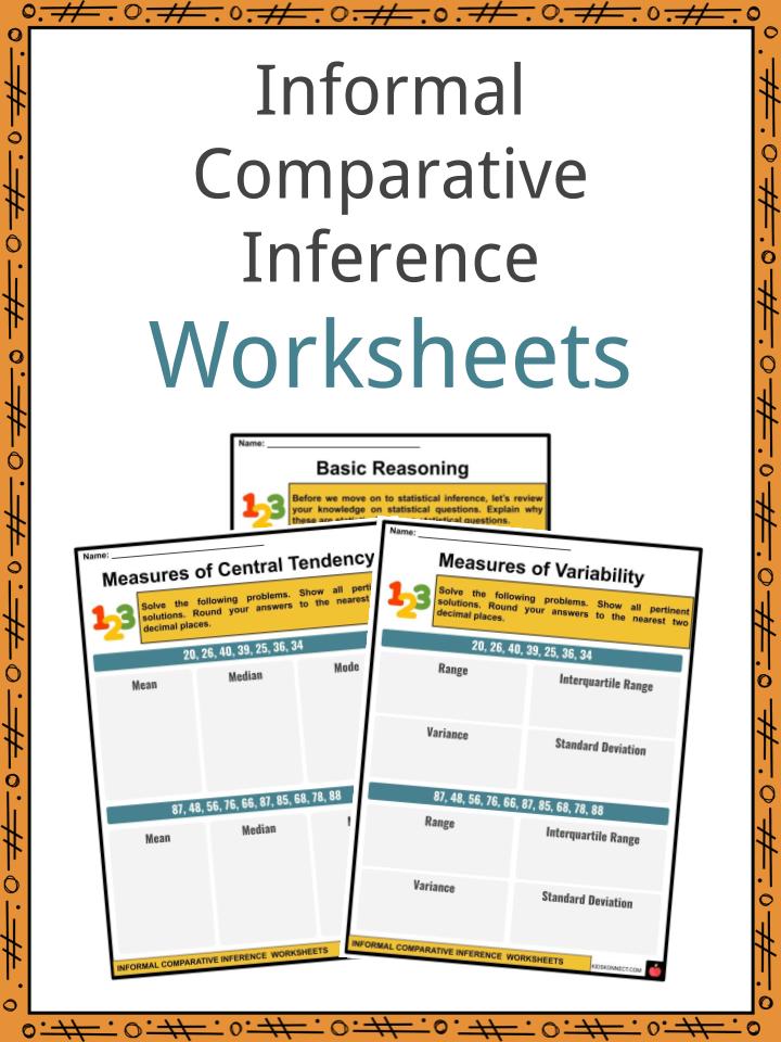
Informal Comparative Inference Worksheets
This is a fantastic bundle which includes everything you need to know about the informal comparative inference across 33 in-depth pages. These are ready-to-use Informal Comparative Inference worksheets that are perfect for teaching students how to draw informal comparative inferences about two populations. They will informally assess the degree of visual overlap of two numerical data distributions with similar variabilities, measuring the difference between the centers by expressing it as a multiple of a measure of variability. Moreover, they will expand their knowledge on the use of measures of center and measures of variability for numerical data.
Complete List Of Included Worksheets
- Lesson Plan
- Informal Comparative Inference
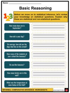
- Basic Reasoning
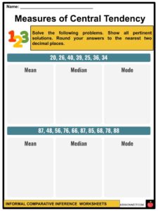
- Measures of Central Tendency
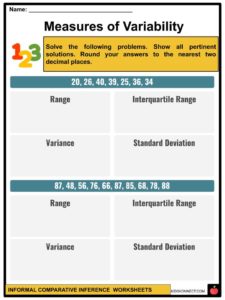
- Measures of Variability
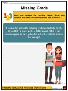
- Missing Grade
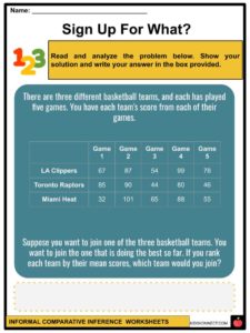
- Sign Up For What?
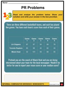
- PR Problems
- Sports Talk
- Sports Talk 2.0
- Two Comic Books
- Test Yourself
Link/cite this page
If you reference any of the content on this page on your own website, please use the code below to cite this page as the original source.
Link will appear as Informal Comparative Inference Facts & Worksheets: https://kidskonnect.com - KidsKonnect, August 1, 2020
Use With Any Curriculum
These worksheets have been specifically designed for use with any international curriculum. You can use these worksheets as-is, or edit them using Google Slides to make them more specific to your own student ability levels and curriculum standards.